Hyperparameter search for scVI

July 5, 2019 · 20 min read

Gabriel Misrachi, Jeffrey Regier, Romain Lopez, Nir Yosef

While stochastic gradient-based optimization is highly successful for setting weights and other differentiable parameters of a neural network, it is in general useless for setting hyperparameters -- non-differentiable parameters that control the structure of the network (e.g. the number of hidden layers, or the dropout rate) or settings of the optimizer itself (e.g., the learning rate schedule). Yet finding good settings for hyperparameters is essential for good performance for deep methods like scVI. Furthermore, as pointed out by Hu and Greene (2019) selecting hyperparameters is nessary in order to compare different machine learning models, especially if those are substantially sensitive to hyperparameter variations.

Generally, hyperparameter search is known to be challenging for the end-user and time-consuming. Therefore, we added in scVI a module based on the Bayesian optimization framework hyperopt. This new feature makes effective use of multiple GPUs and is a ready-to-use solution for tuning hyperparameters in scVI. This blog post presents this feature and investigates how end-users will benefit from it.

Theory : Bayesian Optimization and `Hyperopt`

First and foremost, one needs to carefully select a metric for which to search for optimal hyperparameters, keeping in mind that this one might depend on the downstream task, as explained in Theis et al. (2016). Since we train a generative model, the held-out negative log-likelihood is a natural criterion for model selection. We therefore rely on it for hyperparameters tuning.

Historically, the very first methods introduced to tackle hyperparameter search were grid search and random search. Such approaches are limited in the sense that they scale exponentially with the size of the search space. A more scalable and elegant approach to search is Bayesian Optimization (BO), whose main idea is to learn and use the structure of the objective function. The overall process can be decomposed into two unordered tasks. One is to define a tractable surrogate prior for the underlying black-box objective (e.g., a Gaussian Process). The other is to define a criterion for which to optimize this surrogate process.

In the special case of hyperopt the criterion used is the expectation of the improvement over a certain baseline which can be the current best or lower. The surrogate is called a Tree-strctured Parzen Estimator. The TPE divides the sample set into two subsets based on their value compared to the current baseline and estimates two corresponding conditional densities over the search space using non-parametric kernel-density estimators. Then, good samples should have a high conditional density for improving samples and vice versa.

As suggested in the original article Bergsta et al. (2011), this hyper-optimization process can be used asynchronously by mocking the result for the pending trials with the mean of the available samples. Still, it should be noted that if the budget is a single evaluation per process running in parallel, then a random search should be preferred.

There are a certain number of recent approaches competing with hyperopt. Li et al. (2018) proposes Hyperband: an alternative to BO with bandit-based principled early stopping, which scales better with the number of workers. These can be also combined for trial selection and principled early stopping, as explained in Wang et al. (2018). Interested readers might also take a look at two black-box optimizers based on different paradigms, namely the CMA-ES and DFO-TR algorithms - both have available code. BO enthusiasts can take a look at scikit-optimize as well as Ax, Facebook's brand new pytorch-powered ML platform .

Practice : scVI's autotune module

We are excited to release our new autotune module for scVI, based on hyperopt. We thank hyperopt developers for their maintained codebase as well as their intelligent MongoDb-based communication between workers. Using this new feature on the Cortex dataset is as simple as running the code snippet below.

import logginglogger = logging.getLogger("scvi.inference.autotune")logger.setLevel(logging.DEBUG)
if __name__ == "__main__":    best_trainer, trials = auto_tune_scvi_model(        gene_dataset=dataset,        parallel=True,        exp_key="cortex_test",        max_evals=100,    )

Note that the default behaviour of auto_tune_scvi_model is as follows:

A parameter search space containing the learning rate, the network architecture and the dropout rate is provided.
The objective metric is set to be the held-out log-likelihood of the data computed on a test set which size equals 25% of the whole dataset.
All available GPUs are used.

Of course, the behaviour of the auto-tuning process can be widely customized. For example, one can select the number of CPU processes, the ids of the GPUs to use, one can also input their own hyperparameter search space or even their own objective function. For a more advanced usage, we expose functions to launch your own workers, which could be used to run the search on multiple machines.

Results

In order to evaluate the autotune procedure, we ran it on several standard datasets, directly available using our codebase. Namely, we used the Cortex, Pbmc and Brain Large datasets.

Datasets#

Let us first describe these three datasets in more detail.

CORTEX The mouse cortex dataset from Zeisel et al. (2015) contains 3005 mouse cortex cells and gold-standard labels for seven distinct cell types. We retain the top 558 genes ordered by variance.
PBMC As in the scVI manuscript, we concatenated two datasets of peripheral blood mononuclear cells (PBMCs) from a healthy donor from Zheng et al. (2017). After filtering, we extract 11,990 cells with 3446 genes.
BRAIN LARGE This dataset contains 1.3 million brain cells from 10x Genomics. We retain the 720 most variable genes.

For each of these, we ran our autotune process using a default search space and a budget of 100 trainings. The raw outcome of these experiments can be found here in the form of a table containing the parameters used and the resulting performance.

Runtime information#

We report the runtime metadata of our experiments in Table 1. This should give the user an idea of the time it takes to use our new feature, depending on the size of the dataset, the number of evaluations, the max number of epochs allowed and the number of GPUs available.

Dataset Name	Nb cells	Nb genes	Wall time	Avg epochs	N° of GPUs	Max epoch
cortex	3005	558	9 hours	532	1	1000
pbmc	11990	3346	3 hours	387	16	1000
brain large	1303182	720	21.5 hours	43	16	50

Table 1: Runtime Table for 100 trainings. Wall time is the total time the experiment took. Avg epoch is the average number of epochs per training.

Hyperparameter sensitivity#

Our first concern was to investigate scVI's sensitivity to hyperparameters. One ideal way to investigate this matter would have been to study the variance of the performance for each set of hyperparameters and collapse the runs who are not significantly different before analyzing the remaining representants. As this is too computationally intensive, we instead focus on the ten best and ten worst runs for each dataset.

	marginal_ll	n_layers	n_hidden	n_latent	reconstruction_loss	dropout_rate	lr	n_epochs	n_params	run index
1	1218.52	1	256	10	zinb	0.1	0.01	248	290816	92
2	1218.7	1	128	12	zinb	0.1	0.01	382	145920	80
3	1219.7	1	256	10	zinb	0.1	0.01	365	290816	85
4	1220.06	1	256	10	zinb	0.1	0.01	275	290816	91
5	1223.09	1	128	10	zinb	0.1	0.01	440	145408	83
6	1223.2	1	128	12	zinb	0.5	0.005	703	145920	38
7	1223.53	1	256	10	zinb	0.1	0.001	514	290816	97
8	1223.94	1	128	12	zinb	0.5	0.01	542	145920	74
9	1224.37	1	128	12	zinb	0.5	0.01	524	145920	76
10	1224.37	1	128	12	zinb	0.5	0.01	497	145920	71
91	1554.98	2	64	10	zinb	0.7	0.005	256	80896	45
92	1559.01	5	64	7	nb	0.5	0.0001	457	105088	37
93	1601.53	3	64	10	nb	0.7	0.001	88	89088	15
94	1612.9	4	64	14	zinb	0.7	0.005	71	97792	49
95	1615.22	2	256	9	nb	0.9	0.0001	197	421376	20
96	1746.25	3	128	12	zinb	0.9	0.001	134	211456	52
97	1818.82	1	64	12	zinb	0.9	0.0005	54	72960	60
98	6574.57	1	128	8	zinb	0.5	0.0001	4	144896	61
99	10680.4	5	64	12	zinb	0.3	0.0001	2	105728	1
100	NaN	2	64	6	zinb	0.9	0.0001	31	80384	13

Table 2: Hyperoptimization results for the Cortex dataset.

	marginal_ll	n_layers	n_hidden	n_latent	reconstruction_loss	dropout_rate	lr	n_epochs	n_params	run index
1	1323.44	1	256	14	zinb	0.5	0.01	170	1720320	70
2	1323.88	1	256	8	zinb	0.5	0.01	130	1717248	54
3	1324.12	1	256	14	zinb	0.5	0.01	178	1720320	85
4	1324.18	1	256	8	zinb	0.5	0.01	155	1717248	65
5	1324.2	1	256	15	zinb	0.5	0.01	140	1720832	84
6	1324.23	1	256	8	zinb	0.5	0.005	170	1717248	42
7	1324.24	1	256	14	zinb	0.5	0.01	227	1720320	87
8	1324.25	1	256	8	zinb	0.5	0.01	176	1717248	67
9	1324.29	1	128	15	zinb	0.3	0.01	176	860416	73
10	1324.32	1	256	8	zinb	0.5	0.01	133	1717248	69
91	1347.3	3	64	6	nb	0.7	0.01	285	445440	37
92	1350.02	2	128	13	zinb	0.9	0.001	350	892672	8
93	1350.54	1	64	5	zinb	0.9	0.0005	492	428928	0
94	1350.59	1	128	13	nb	0.9	0.01	55	859904	5
95	1350.9	2	128	13	zinb	0.9	0.0005	710	892672	15
96	1352.32	3	256	14	zinb	0.9	0.01	201	1982464	88
97	1355.68	3	256	5	zinb	0.9	0.001	668	1977856	49
98	1365.46	3	256	10	zinb	0.9	0.01	42	1980416	75
99	1367.7	2	128	15	zinb	0.9	0.0001	999	893184	13
100	1370.3	3	256	8	nb	0.9	0.01	55	1979392	81

Table 3: Hyperoptimization results for the Pbmc dataset.

	marginal_ll	n_layers	n_hidden	n_latent	reconstruction_loss	dropout_rate	lr	n_epochs	n_params	run index
1	1143.79	1	256	15	zinb	0.1	0.0005	50	376320	92
2	1144.11	1	256	15	nb	0.1	0.0005	42	376320	72
3	1144.22	1	256	14	nb	0.1	0.005	48	375808	70
4	1144.84	1	256	14	nb	0.1	0.005	43	375808	86
5	1144.97	1	256	14	nb	0.1	0.005	48	375808	68
6	1145.08	1	256	14	nb	0.1	0.005	43	375808	51
7	1145.2	1	256	14	nb	0.1	0.005	47	375808	85
8	1145.86	2	256	13	nb	0.1	0.0001	49	506368	55
9	1146.05	2	256	13	nb	0.1	0.0001	49	506368	42
10	1146.11	2	256	13	nb	0.1	0.0001	49	506368	58
91	1185.27	5	128	13	zinb	0.5	0.0005	49	318720	40
92	1188.06	5	256	14	nb	0.7	0.0001	44	900096	24
93	1188.98	4	128	15	nb	0.5	0.005	49	286464	4
94	1193.21	5	256	8	zinb	0.7	0.005	47	897024	30
95	1202.7	5	128	11	nb	0.5	0.001	46	318208	11
96	1203.35	2	64	13	nb	0.7	0.0001	49	102016	56
97	1205.6	2	64	9	nb	0.7	0.0001	48	101504	82
98	1206.69	4	128	12	nb	0.7	0.0001	47	285696	61
99	1211.31	5	256	7	nb	0.7	0.005	38	896512	74
100	1232.12	5	64	15	nb	0.7	0.0001	26	126848	52

Table 4: Hyperoptimization results for the Brain Large dataset.

From Table 2, 3 and 4 we note that the obtained parameters agree on certain aspects such as the number of layers or the learning rate. Additionally, it is worthwhile noting that the best results often come from configurations with the maximal number of hidden neurons (256), in particular for the PBMC and Brain Large datasets. Perhaps, better performance could be obtained by increasing the search space on this component.

We purposedly do not use these results to conclude on which type of conditional distribution for the count distribution (NB, ZINB or other; parameterized by reconstruction_loss). Surprisingly, another tuning process run on the PBMC dataset consistently selected the negative binomial loss in the ten best runs. This likely is a bias introduced by the exploration process during the optimization procedure. See our group's blog post by O. Clivio and P. Boyeau for a complete analysis of the conditional distribution choice.

Overall, the best performances are stable even though we notice that small changes can have large impacts when we look at the full results (e.g, the number of layers can lead to a sensible difference in held-out log-likelihood). Such stability is in accordance with our extended use of scVI and scANVI in our harmonization preprint Xu et al. (2019), where we keep the hyperparameters fixed and obtain competitive performance with state-of-the-art methods. However, we recognize that hyperparameter tuning is an important practice in machine learning method developements and benchmarking and advocate the use of our autotune module for model selection and comparaisons.

The case of the Brain large dataset#

Given the amount of data available for this dataset, we were expecting to reach optimality with more hidden layers in our neural networks (as shallow networks with bounded width represent a potentially small function class). Suprisingly enough, single-hidden-layer models came out as the best contenders. In Figure 1, we investigate in further details the relationship between our n_layers parameter and the observed performance in terms of marginal negative log-likelihood.

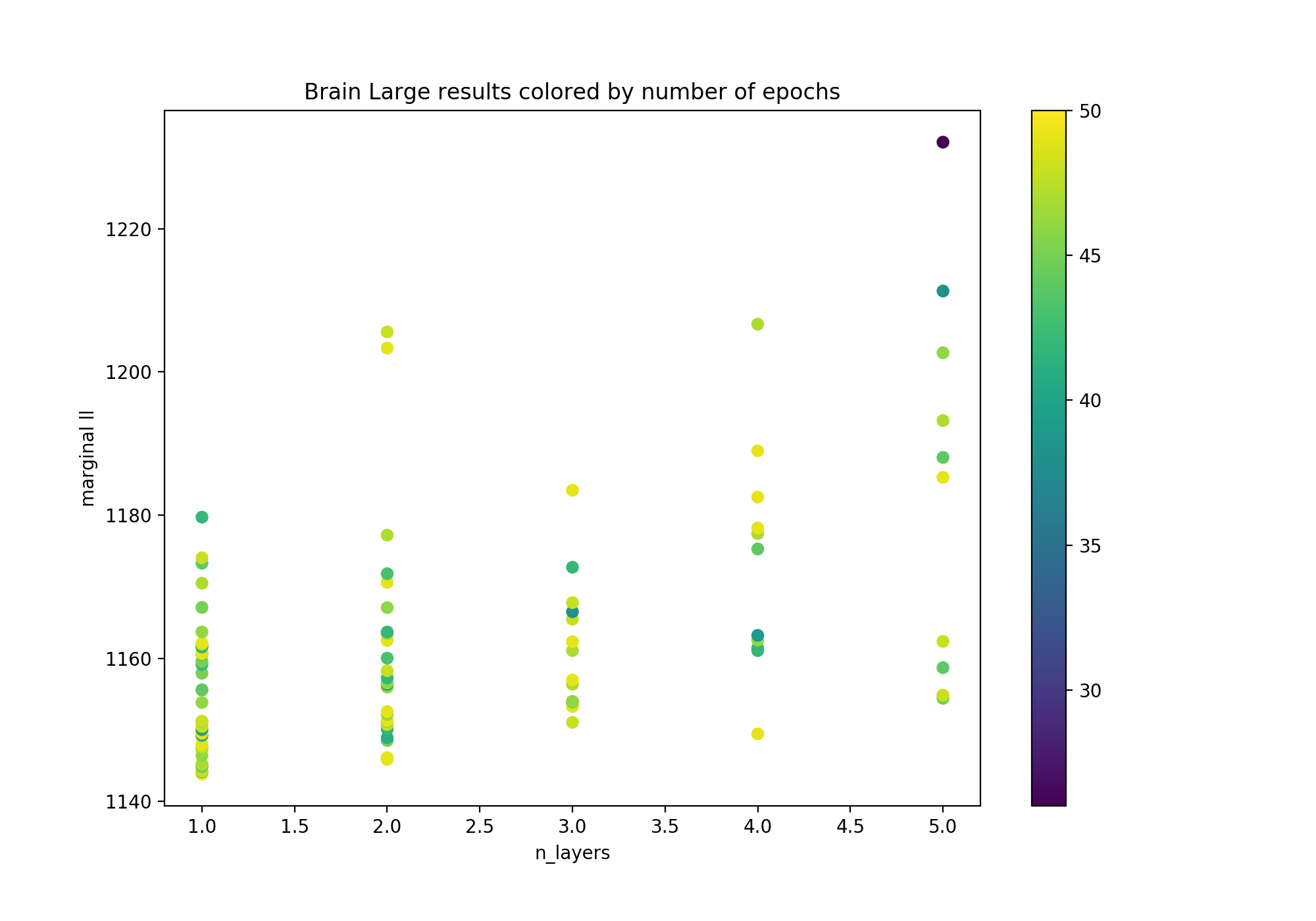
Figure 1: Marginal negative log-likelihood as a function of the number of hidden layers in scVI's encoder/decoder, colored by the number of epochs. The number of epochs was limited to 50 or less if the early stopping criterion was triggered.

It is clear from Figure 1 that the shallow versions of scVI reach better performances on average. Still, a significant portion of hyperparameter configurations reach the maximum number of epochs. Potentially, allowing for a higher budget in terms of the number of epochs could change the outcome of our experiment. Additionally, the fact that we keep only the 720 most variable genes may be too big of a restriction on the amount of signal we keep, making this filtered version of the dataset simple enough to be better and faster captured by a single-hidden-layer model.

Benchmarking#

Our next concern was to investigate the kind of performance uplift we could yield with auto-tuning. Namely, we investigated how optimizing log likelihood could increase other metrics like imputation for example. Our results are reported in the table below.

Dataset	Run	Likelihood			Imputation score
		Marginal ll	ELBO train	ELBO test	Median	Mean
cortex	tuned	1218.52	1178.52	1231.16	2.08155	2.87502
	default	1256.03	1224.18	1274.02	2.30317	3.25738
pbmc	tuned	1323.44	1314.07	1328.04	0.83942	0.924637
	default	1327.61	1309.9	1334.01	0.840617	0.925628
brain large	tuned	1143.79	1150.27	1150.7	1.03542	1.48743
	default	1160.68	1164.83	1165.12	1.04519	1.48591

Table 5: Comparison between the best and default runs of scVI on the Cortex, Pbmc and Brain Large datasets. Held-out marginal log-likelihood and imputation benchmarks are reported.

Note that the median (resp. mean) imputation score is the median (resp. mean) of the median absolute error per cell. Also, the held-out marginal negative log-likelihood is an importance sampling estimate of the negative marginal log-likelihood $-\log p(x)$ computed on a 25% test set and is the metric we optimize for.

From Table 5, we see that the tuning process improves the held-out marginal negative log-likelihood on all three datasets. This model improvement, in turn, ameliorates the imputation metrics for all three datasets, albeit not significantly for the Pbmc and Brain Large datasets.

Efficiency of the tuning process#

Our last concern was to investigate the efficiency of the tuning process. To do so we wanted to check how the held-out negative Evidence Lower BOund (ELBO) histories of the runs were evolving with the number of runs. Below is a plot of these histories.

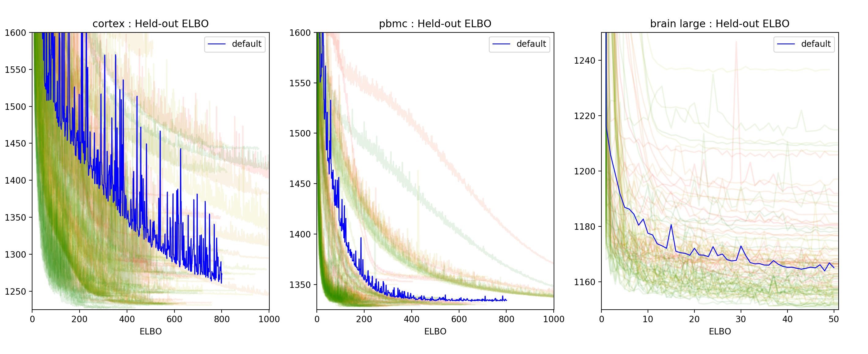
Figure 2: Held-out negative ELBO history for each of the 100 trainings performed for each dataset. The lines are colored from red to green where red represents the first trial and green the last one.

In Figure 2, we see that most green runs (the last trials) are concentrated in the low negative ELBO regions which indicates that the TPE algorithm provides relevant trial suggestions. This would suggest that allowing a slightly higher budget might yield better results. The user should consider this when setting the number of evaluations to run.

Discussion

As we illustrated, hyper-parameter tuning provides a improvement for the data fit and also for any metrics that are correlated with the held-out marginal log-likelihood. It is possible that some other scores such as clustering might not be improved by this process since scVI is not per se separating any form of clusters in its latent space. A case where improvement on log-likelihood should be correlated with better clustering scores is for example when using scANVI, which has a Gaussian mixture model prior over the latent space.

In this set of experiments, the hyperparameter selection procedure retained for all datasets an architecture with a unique hidden layer. To make sure that scVI benefits from non-linearity (compared to its deterministic homolog ZINB-WaVE), we investigated whether hyperopt would select a model with one layer compared to a linear model. We report our results in this table and conclude that a non-linear model sensibly outperforms the linear alternative on both of the Cortex and Pbmc datasets. Brain Large was not part of this experiment as it would have required a considerable amount of additional computing ressources. Besides, it is worth mentioning that some contemporary results tend to indicate that deep architectures are good approximators for gene expression measurements. For instance, Chen et al. (2016) compare linear regression to their deep neural network D-GEX on gene expression inference. They show architectures with three fully-connected layers outperform shallower architectures and linear regression by a significant margin. Such evidence could very well motivate a more in-depth study of scVI's optimization procedure. Perhaps, techniques to improve and accelerate deep neural-networks training could have a significant impact on the results we are able to reach. For example, between-layer connections such as those proposed in the DenseNet architecture Huang et al. (2018) might lead a path towards future improvement. In the meantime, we also plan to release a patch to scVI allowing for assymetric encoders and decoders as well as variable number of hidden units for each layer of each of scVI's neural networks.

Finally, we have seen how sensible scVI can be with respect to its set of hyperparameters on certain datasets. Thus, our new hyperparameter tuning feature should be used whenever possible - especially when trying to compare other methods to scVI. We note Qiwen Hu and Casey Greene's remarks on hyperparameter selection as well as their comment on Nature Methods and aknowledge their work being our main motivation for incorporating this new tool into scVI.

Acknowledgements

We acknowledge Valentine Svensson for proposing the linear decoder and contributing to the scVI codebase.