Should we zero-inflate scVI?

Droplet- based single-cell RNA sequencing (scRNA-seq) datasets typically contain at least 90% zero entries. How can we best model these zeros? Recent work focused on modeling zeros with a mixture of count distributions. The first component is meant to reflect whether such an entry can be explained solely by the limited amount of sampling (on average ~5% or less of the molecules in the cell). The second component is generally used to reflect "surprising" zeros caused by measurement bias, transient transcriptional noise (e.g., "bursty" gene with a short mRNA half life), or true longer-term heterogeneity that can not be captured by a similified (low dimensional) representation of the data. Among others, zero-inflated distributions (i.e., zero-inflated negative binomial) have been widely adopted to model gene expression levels (1, 2).

Recently, some have questioned the zero-inflated nature of scRNA-seq data (3, 4). For instance, it can be shown that negative binomials alone are sufficient to properly model variations of negative control droplet-based scRNA-seq data, for which there is no biological variation. These results suggest that the majority of zeros in the data can be explained by low sampling rate (i.e., low capture efficiency exacerbated by limited sequencing depth). However, there may still be motivation to model additional zeros as gene or cell-specific technical effects. Finally, some of these dropout events might be of different biological nature. Such a scenario is especially motivated by the bursty transcriptional kinetics model, which when coupled with limited sensitivity, could contribute to added observed zeros (or a more complicated, bimodal distribution). Whether such bursty model can be estimated from scRNA-seq data is a challenging question, with promising recent results that are based on allele specificity (5).

In this blog post, we adopt a purely computational, data-driven approach to investigate whether scRNA-seq data is zero inflated. In particular, we rely on Bayesian model selection rules to determine for a given list of scRNA-seq datasets whether a zero-inflated model can fit the data significantly better. We propose to use two natural criterions for model selection: held-out log likelihood (as in (6)) and posterior predictive checks (PPCs, as in (7)). Finally, the optimal distribution could in principle depend on the gene set and even be gene-specific within a given gene set. We therefore propose a metric to underline how much individual genes are better fitted by zero-inflated distributions.

Methodology

Models

The original scVI (1) model (referred to as the ZINB model) uses a zero-inflated negative binomial (ZINB) likelihood to model gene expression counts. In particular, the dropout probability $p_{ng}$ for each cell $n$ and each gene $g$ is learned via a neural network $\hat p_{ng} = f_h^g(z_n)$. We compare this ZINB model to scVI modified to instead use a negative binomial likelihood (referred to as the NB model). The NB model is equivalent to setting $p_{ng}$ to zero.

Model selection metrics

For model selection, we first consider held-out log likelihood. The marginal log-likelihood for our model is intractable. However, we can estimate it through importance sampling, with our variational distribution as the proposal distribution. In our tables of results, we report a Kolmogorov-Smirnov statistic, hence lower is better. More details can be found in Appendix A. In addition, although this is not a metric for model comparison, we report for each dataset under scrutiny the average over all cell-gene entries of the dropout probabilities computed by the ZINB model and we report it as "ZINB dropout".

Hyperparameters selection

Some concerns can be that a model's hyperparameters play a significant part in its performance and that improper tuning might affect our analysis. As a result we performed hyperparameters tuning on all datasets that we have considered using scVI's new autotune module, based on the hyperopt package. The hyperparameters were selected to maximize held-out log-likelihood, and we used early stopping. We refer to the blog article by Gabriel Misrachi which introduces this new scVI module.

Statistical significance

Although the number of samples used in PPCs computations did not influence much the variance of the results, we noticed that the initialization of scVI's neural nets weights could have a high impact on the value of the evaluation metrics. All experiments are hence run 100 times. Each metric is saved for all runs. We use a two-sample one-sided Wilcoxon rank-sum test with a $0.05$ significance level on each of the selected metrics for all the random initializations to decide whether one model is better than another. A model estimated to significantly outperform the other one is marked as bold in our tables of results.

Finding zero-inflated genes

We also tried to predict which genes were zero-inflated. For this purpose, we assigned each gene a score based on the difference of reconstruction loss of the model for the best ZINB and NB models. We then interpret genes with high positive scores as "zero-inflated" genes.

Results

Datasets

We consider a mixture of synthetic datasets from multivariate count distributions (Appendix B), real datasets with spike-in measurements (analyzed in (3)) and real datasets (analyzed in (1) and accessible from the scVI codebase).

Dataset name	Cells	Protocol
ZISynth	12,000	Synthetic data, see Appendix B
Klein et al. 2015 (13)	953	InDrops
Zheng et al. 2017 (11)	1,015	GemCode
Svensson et al. 2017 (1) (3)	2,000	10x Chromium (v1)
Svensson et al. 2017 (2) (3)	2,000	10x Chromium (v1)
Brain Small (11)	9,128	10x Chromium (v2)
Cortex (9)	3,005	Smart-Seq2
Hemato (10)	4,016	InDrops
PBMC (11)	12,039	10x Chromium (v2)
Retina (12)	27,499	Drop-Seq

The synthetic datasets served as a sanity check that our methodology made sense on data that we had ground truth for. We selected these datasets to validate that our metrics are consistent whether or not the data is zero-inflated. The datasets from (3) were restricted to ERCC spike-ins who were present in more than 20% of the data. Cortex, Hemato, Brain Small, Retina, PBMC were restricted to the 1200 most variable genes to speed-up computations.

Results on synthetic datasets

We first analyze the results on the ZISynth dataset for different values of the parameter $\lambda$ that controls zero-inflation. As detailed in Appendix B, the probability for a given entry $x_{ng}$ to be zero-inflated is $p_{ng} = pe^{-\lambda x_{ng}^2}$ where $p = 0.08$ and $\lambda > 0$ is a user-defined parameter. The setting $\lambda = 0$ corresponds to a uniform dropout, $\lambda \rightarrow \infty$ to the absence of zero-inflation and $0 < \lambda < \infty$ to an intermediate regime where the dropout probability for each cell-gene is a decreasing function of its expression. The results are shown in Table 1.

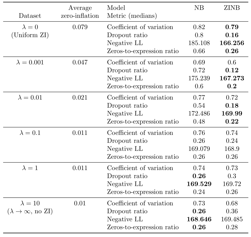
Table 1: Results of the Bayesian model selection experiments on synthetic data.

We note several things. First, for $\lambda = 0$, or the uniform dropout regime, the ZINB model significantly outperforms the NB model. Moreover, the average computed dropout probability for the uniform ZI model is in the range $0.075-0.08$ depending on the simulation, which is coherent to the ground truth dropout probability ($0.08$). Hence, a uniformly zero-inflated dataset seems better explained by a zero-inflated model.

For $\lambda \rightarrow \infty$ (obtained in practice with $\lambda = 10$), the NB model significantly outperforms the ZINB model on almost all metrics, except the coefficient of variation where there is a tie. Moreover, the average estimated dropout probability for the ZINB model is in the range $0.0073 - 0.011$ depending on the simulation, proving than no zero-inflation is probably a better solution compared to even a very small zero-inflation on such a dataset. It also ensures that the metrics are not biased in favor of zero-inflation.

For $0 < \lambda < \infty$, as $\lambda$ increases, we note that the number of metrics where the ZINB model significantly outperforms the NB model tends to decrease whereas the number of metrics supporting the opposite tends to decrease. Hence, increasing $\lambda$ from 0 to $\infty$ marks a transition from an uniformly zero-inflated dataset to a non-zero-inflated dataset. The value of $\lambda$ where zero-inflation may stop to be needed is located between $\lambda = 0.1$ and $\lambda = 1$.

Studying the zeros of synthetic datasets

For each entry of the data matrix (cells x genes), the ZINB model jointly learns the average of the NB distribution and the dropout probability. In the scVI manuscript, we searched for correlation between dropout probabilities and quality control metric of individual cells (1) (Supplementary Figure 13). In this work, we focus instead on the distributions of inferred NB means and dropout probabilities for the zero entries of our synthetic dataset. In this test, we use simulation to investigate two categorical "types" of zeros in the data. The first group of zeros are the result of limited-sampling. The chance to have a zero of this type is negatively correlated with the negative binomial mean. Ideally, limited-sampling zeros can be captured by the negative binomial component alone. The second type of zeros, which we refer to as dropout, are introduced as zeros that would require zero-inflation from scVI. These zeros can be introduced uniformally ($\lambda=0$) regardless of the expression level of the respective gene, or depend on the expression levels ($\lambda > 0$). In the following we tested whether scVI can distinguish those two types in an unsupervised fashion and whether the parameters of interest (i.e., inferred NB mean and inferred dropout probability) are interpretable. We report such results in Figure 1 for different values of the $\lambda$ parameter (further experimental details in appendix C).

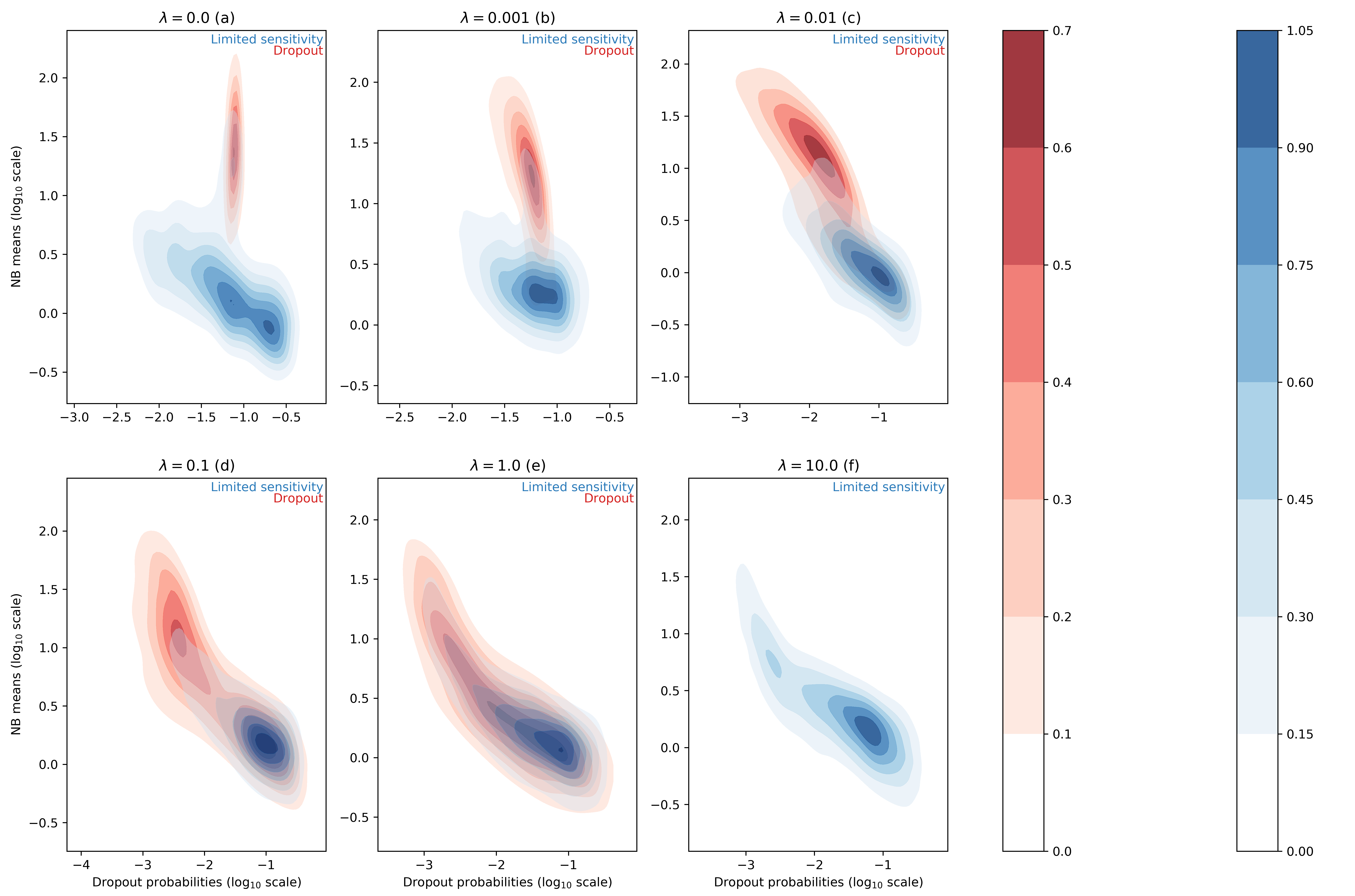
Figure 1 : distributions of estimated dropout and NB means for different ZISynth datasets. In blue, the points corresponding to limited-sampling zeros. In red, the points corresponding to dropout zeros.

For the uniformly zero-inflated dataset (Figure 1a) we can observe that the dropout probability and NB mean are anti-correlated : the higher the dropout probability, the lower the NB mean. This contradicts the possible expectation that the predicted NB mean would compensate a high predicted dropout with a higher value. One can note that scVI successfully captures the uniform dropout distribution, as the bulk of predicted dropout probabilities on dropout entries - generated from a uniform dropout $p_{ng} = 0.08$ probability - is located around a value close to the associated ground-truth value, as $10^{-1.1} \approx 0.8$. On the other hand, the bulk of scVI's predicted zero-inflation probabilities $\hat p_{ng}$ associated to the limited-sampling zeros is also located around a value close to $0.08$, although with a higher dispersion. Such a behavior is explained by the fact that in scVI, the neural net $f_h^g$ (refer to (1)) predicts the dropout rate from $z_n$. However, in the case of uniform dropout, $p_{ng}$ do not depend on this variable and therefore $f_h^g$ learns a constant value equal to $0.08$.

If we consider the non-uniformly zero-inflated (Figures 1b-1e) or non-zero-inflated (Figure 1f) datasets we note that the predicted dropout for dropout zeros now follows a similar distribution than for limited-sensitivity zeros since the NB mean now tends to decrease with the dropout probability which is no longer confined around a fixed value. Hence, despite relying on the latent variable $z_n$ and not on the expression $x_{ng}$ for each cell-gene, the ZINB model can still learn the structure of an injected dropout clearly defined as decreasing with the cell-gene expression. The higher the parameter $\lambda$, the closer the distributions of NB means and dropout probabilities are between limited-sensitivity and dropout zeros. In the end, and as a sideline, for $\lambda = 10$ the dropout zeros disappear as there is no more zero-inflation, as explained previously. The limited-sensitivity zeros still tend to have a higher dropout probability than dropout zeros, which is a clear point to study in further developments of scVI. Note : the same plots using the total probability of zero instead of the dropout probability (Figure 1bis) can be found in appendix C.

Results on ERCC spike-in measurements

We focus on the datasets that contains only synthetic RNA transcripts (ERCCs) and report the results in Table 2. Regarding the ERCC spike-in datasets in (3), the distribution of zeros of all of them seems better modelled without zero-inflation, as expected from the paper. Only for Svensson et al. 2017 (2) does a metric support ZINB instead of NB (the coefficient of variation). However, investigations on the computed dropout probabilities show that the average dropout dropability for this dataset is located between 0.02 and 0.03, which indicates that the zero-inflation is not very influencial. Meanwhile, the average dropout probability is greater than 0.05 on the three other datasets from (3) and greater than 0.09 on the five biological datasets discussed in the next paragraph, which indicates a more significant effect of zero-inflation and shows that the comparison between a NB model and a ZINB model is not superfluous.

We note that some metrics are shown to significantly support either NB or ZINB when medians for both models or equal; this is due to better ranks in general on the whole distribution for the model designated as better performing.

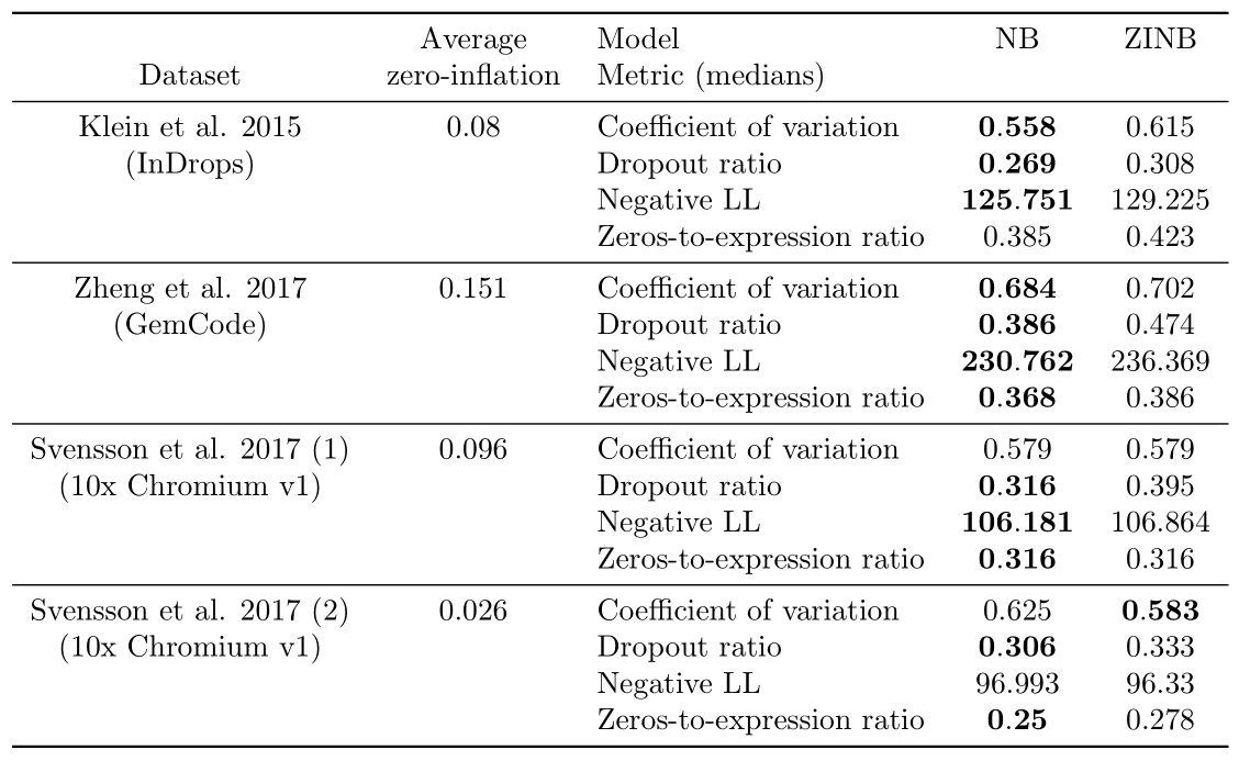
Table 2: Results of the Bayesian model selection experiments on the spike-in datasets.

Results on real datasets

We report results on the real datasets in Table 3.

On the Cortex dataset, the ZINB model performs better than the NB model on all metrics except the zeros-to-expression ratio where there is a tie, showing that zero-inflation may be adapted to this dataset. On the Hemato dataset, ZINB may fit better the data, as shown by the two metrics where it significantly outperforms NB. The difference is much less significant on dropout-related metrics however. On the Brain Small dataset, the ZINB model performs better than the NB model on all metrics except the negative log-likelihood where there is a tie. This suggests that zero-inflation may help capture both the distribution of zeros and variability better. For the PBMC dataset, there is a tie, as the NB model demonstrates a better performance with regards to coefficient of variation and the ZINB model performs better on negative log-likelihood, whereas both dropout metrics do not support either NB or ZINB. Finally, on the Retina dataset, the ZINB model may provide a better fit, as shown by the negative log-likelihood metric where it significantly outperforms NB but similarly as Hemato, the difference is much less significant on dropout-related metrics, and it is also very small on the coefficient of variation PPC metric.

For each dataset, we also report the empirical proportion of zero entries in the matrix as well as the average dropout probabilities returned by the ZINB model. As expected, all of the droplet-based sequencing datasets have more frequent zero entries than the Smart-seq2 dataset. However, we notice that Cortex (Smart-Seq2) has a high average dropout probability, which suggests that a non negligible fraction of the zeros could be attributable to zero inflation. Such a result is compatible with recent hypotheses that PCR duplication or uneven fragment sampling may be responsible for zero-inflation in plate-based technologies (3). Among all the others droplet-based sequencing datasets, we see that Hemato (InDrops) and Retina (DropSeq) have an high average dropout probability when compare to Brain Small and PBMC (10x Chromium v2). Such discrepencies might be attributable to either more biological variability in these specific datasets, or the quality of the experimental assay. In future work, we will examine whether such results are consistent across datasets of the same technology and study more experimental protocols.

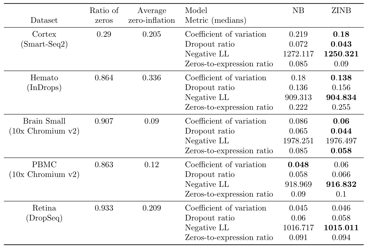
Table 3: Results of the Bayesian model selection experiments on Cortex, Hemato, Brain Small, PBMC and Retina.

Finding zero-inflated genes

We report an histogram of gene-specific reconstruction loss discrepencies for the Hemato dataset in Figure 2. As shown below, gene zero-inflation scores have heavy tails, corresponding to genes for which one or the other hypothesis makes more sense than the other. Non-exhaustive lists of predicted ZINB or NB genes are provided in appendix D.

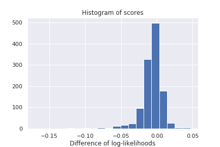
Figure 2: Histogram of gene-specific reconstruction loss discrepencies between ZINB and NB model on the Hemato dataset

Conclusion

This study explored whether adding zero-inflation to a negative-binomial likelihood improves the scVI model. Results on synthetic datasets show our metrics enable a fair comparison between the two zero-inflated and non-zero-inflated models. Results on real datasets show that zero-inflation is helpful for many existing scRNA-seq datasets, although not all.

Naturally, a more complex distribution is suitable only if it proves to fit the data better (at least empirically). We pursued in this blog a discussion about dropout events and limited sensitivity zeros which has the merit to shed light on how scVI fits this ZINB distribution to the data. Since in practice it is impossible to perfectly disentangle technical noise and biological signal, it would be interesting to extend the analysis to scenarios where the dropout is indeed biological (e.g., transcriptional bursting model).

Please share any feedback with us via twitter (@YosefLab) or through the comment section below.

Acknowledgements

We acknowledge members of the Yosef Lab, especially Zoë Steier and Matt Jones for remarks on some of the results on this blog post. We thank Adam Gayoso for reviewing some of the code and Gabriel Misrachi for his work on scVI's new autotune module, which is the basis for meaningful model selection.

Bibliography

(1) Romain Lopez, Jeffrey Regier, Michael B Cole, Michael I Jordan, and Nir Yosef. Deep generative modeling for single-cell transcriptomics. Nature Methods, 2018.

(2) Emma Pierson and Christopher Yau. ZIFA: Dimensionality reduction for zero-inflated single-cell gene expression analysis. Genome biology, 2015.

(3) Valentine Svensson. Droplet scRNA-seq is not zero-inflated. biorXiv, 2019.

(4) Beate Vieth, Christoph Ziegenhain, Swati Parekh, Wolfgang Enard, and Ines Hellmann. powsimR: poweranalysis for bulk and single cell RNA-seq experiments. Bioinformatics, 2017.

(5) Larsson, A.J.M., et al. Genomic encoding of transcriptional burst kinetics, Nature, 2019.

(6) Christopher Heje Grønbech, Maximillian Fornitz Vording, Pascal Timshel, Casper Kaae Sønderby, Tune Hannes Pers, and Ole Winther. scVAE: Variational auto-encoders for single-cell gene expression data. bioRxiv, 2019.

(7) Hanna Mendes Levitin, Jinzhou Yuan, Yim Ling Cheng, Francisco JR Ruiz, Erin C Bush, Jeffrey NBruce, Peter Canoll, Antonio Iavarone, Anna Lasorella, David M Blei, and Peter A Sims. De novo gene signature identification from single-cell RNA-seq with hierarchical Poisson factorization. Molecular Systems Biology, 2019.

(8) Brian H. Neelon, A. James O’Malley, and Sharon Lise T. Normand. A Bayesian model for repeated measures zero-inflated count data with application to outpatient psychiatric service use. Statistical Modelling, 2010

(9) Zeisel, A. et al. Cell types in the mouse cortex and hippocampus revealed by single-cell rna-seq. Science 347, 1138–1142, 2015

(10) Tusi, B. K. et al. Population snapshots predict early haematopoietic and erythroid hierarchies. Nature 555, 54–60, 2018.

(11) Zheng, G. X. Y. et al. Massively parallel digital transcriptional profiling of single cells. Nature Communications 8, 14049, 2017

(12) Shekhar, K. et al. Comprehensive classification of retinal bipolar neurons by single-cell transcriptomics. Cell 166, 1308–1323.e30, 2017.

(13) Klein, A.M., et al. Droplet barcoding for single-cell transcriptomics applied to embryonic stem cells. Cell 161, 1187–1201, 2015

Appendix A: Posterior Predictive Checks details

Posterior predictive checks (PPCs) are another way to assess Bayesian models. The idea is to check if data simulated from the posterior predictive distribution of a model matches what we observe on real data. The exact pipeline we followed, adapted from (6) can be described as:

Evaluation procedure

• Generate synthetic data matrix $\hat x$ from the posterior predictive of the criticized model. The posterior predictive is sampled 100 times.

• Construct a discrepancy measure $T$ meaningful of the context and compute $\hat T_g = T(\hat x_{g})$ for each gene and each of the 100 samples of the posterior predictive, before averaging on these samples. Several choices of $T$ can make sense, described in a coming paragraph. In parallel, the ground truth discrepancy measure $T^0_g = T(x_g)$ from real training data is computed.

• We now have at disposal $S:=\{\hat T_g, g \in \mathcal{G}\}$ and $S^0:=\{T_g^0, g \in \mathcal{G}\}$ the set of synthetic and real observations of the discrepancy measures. A non-parametric test (2-sample Kolmogorov-Smirnov) is then applied. The obtained KS statistic is $K = \sup d(F_n , F_n^0)$, where $F_n$ and $F_n^0$ are the empirical distribution functions of $S$ and $S_0$ can be understood as a metric describing how different the synthetic and real distributions of measures are. In our experiments, $d$ is the absolute value.

Designing the discrepancy measure

Keeping in mind that we want to determine if the Negative Binomial can on its own explain the important number of zeros of scRNA data, a natural choice of T can be the dropout ratio - the fraction of zeros in the gene expression matrix (averaged over cells, for a specific gene). Another measure could be the zeros-to-expression ratio - the ratio of the number of zeros to the mean of non zero gene expressions (over all cells for a specific gene). Finally, the coefficient of variation defined as the standard deviation of gene expressions divided its mean can be a judicious choice as it is a standard metric in biology (8).

Appendix B: Generative process for simulated data

In practice, we faced some difficulties to observe coherent results at first on (zero-inflated) negative binomial data. Indeed, while zero-inflated synthetic data was most of the time better explained by ZINB-scVI with regards to our metrics, we observed that NB-scVI was not significantly better at explaining non-inflated data with enough examples. On such data, ZINB-scVI had very low predicted dropout probabilities, less than $0.005$, hence approaching NB-scVI and making it difficult to show that NB-scVI was a better choice even in this case. As a consequence, we decided to generate data following a Poisson-LogNormal process, which is another popular distribution to model scRNA gene expressions (2).

We assume there are 2 cell clusters and that every cell $n \in \{1, 2\}$ is an independent replicate of the following generative process. Let $\pi$ a vector in the $1$-dimensional simplex describing the proportion of cells from each cell type, for instance $\pi = (0.70,0.30)$ . Latent variable $c_n \sim Cat(\pi)$ designates the type of cell $n$. Let $\mu_c$ (resp. $\Sigma_c$) be a 50-dimensional vector (resp. 50 $\times$ 50 covariance matrix) for each cell type $c$. Latent variable $z_n \sim \textrm{LogNormal}(\mu_{c_n}, \Sigma_{c_n})$ represents the average expression vector for cell $n$. Finally, we observe for each cell $n$ and gene $g$ the random variable $x_{ng} \sim \textrm{Poisson}(z_{ng})$. $\mu_c$ and $\Sigma_c$ were fitted from a real scRNA-seq dataset.

The dataset ZISynth relies on the latter process, but by also adding zero-inflation by multiplying each gene expression $x_{ng}$ by $h_{ng} \sim Ber(1 - p_{ng})$ where $p_{ng} = pe^{-\lambda x_{ng}^2}$, $p$ being a fixed constant dropout probability, set at $p = 0.08$, and $\lambda \geq 0$ is a hyperparameter. Hence, when $\lambda > 0$, the higher the gene expression, the lower probability it has to be zeroed. $\lambda = 0$ corresponds to a uniform zero-inflation. Finally, $\lambda \rightarrow \infty$ corresponds to the absence of zero-inflation, as the dropout probability is nonzero if and only if the entry is already zero. In practice, in our simulations, $\lambda = 10$ proved enough to attain that regime.

Appendix C: Zeros of scVI - supplementary methods

To generate these figures, we trained ZINB-scVI with its optimal parameters - estimated with hyperopt - for each dataset under scrutiny. From that, we infer the NB mean and the dropout probability on each cell-gene entry 100 times before averaging them on the 100 inferences, again for each cell-gene entry. On the other hand, we retrieve the locations of limited sensitivity zeros and dropout using pre-computed class attributes, and we restrict the average NB means and dropouts to these zero entries.

Generating the same plots with the total zero probability instead of the dropout probability leads to the following figures, hence to similar conclusions.

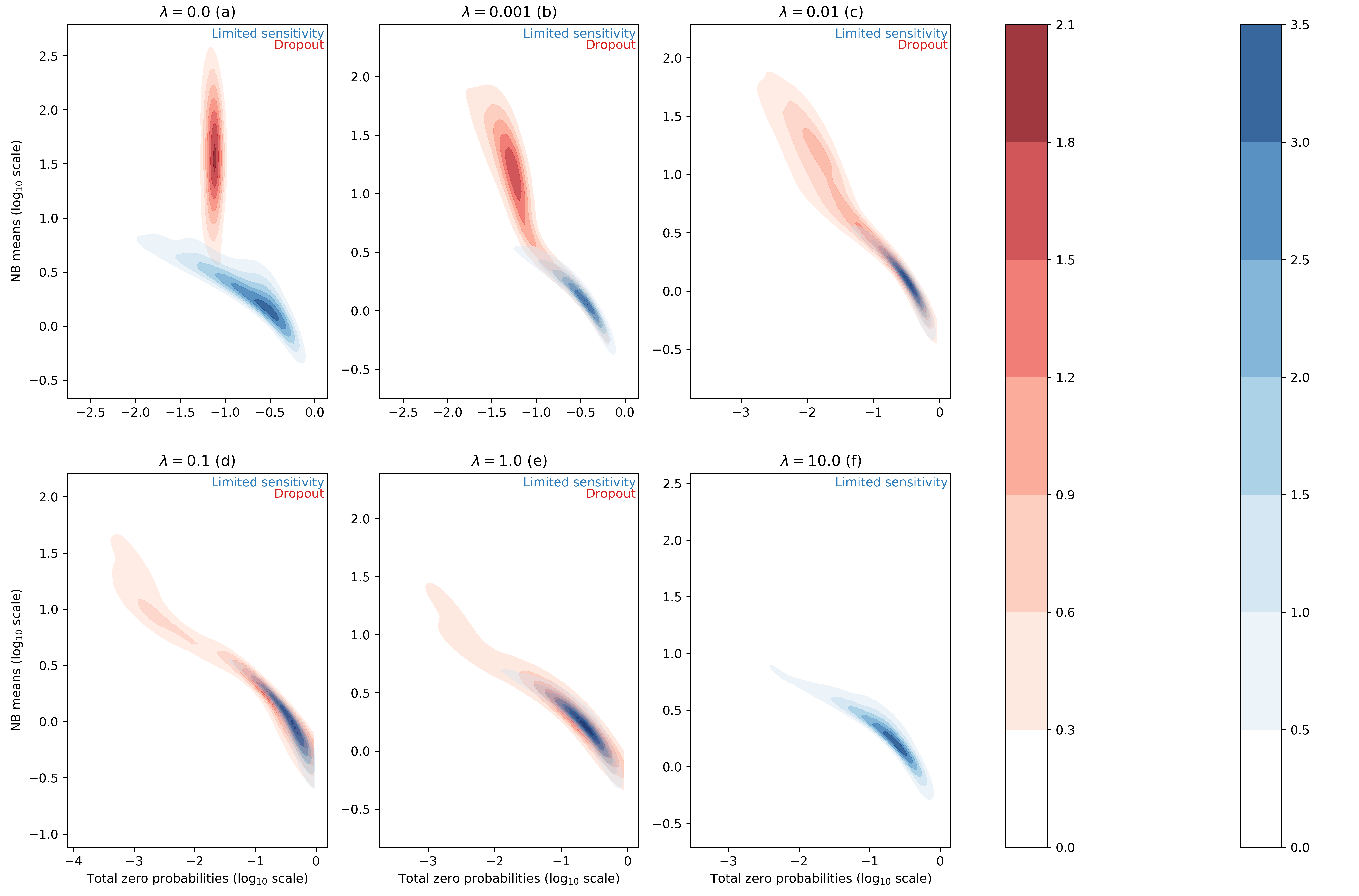
Figure 1bis : distributions of estimated total zero probabilities and NB means for different ZISynth datasets

Appendix D: Zero-inflated genes

Zero-Inflated genes (HEMATO Dataset)

gene	score
Ube2c	-0.17
Plk1	-0.122
Mki67	-0.119
Irf8	-0.098
Ifitm1	-0.095
Racgap1	-0.092
Tuba1c	-0.08
Lmo4	-0.078
Nusap1	-0.074
H2-Aa	-0.073

Zero-Inflated genes (CORTEX Dataset)

gene	score
APOD	-0.254
CALM3	-0.207
GRIA1	-0.174
SYT1	-0.17
SCN2A1	-0.169
CELF2	-0.168
KIF5C	-0.163
XIST	-0.162
GRIN2B	-0.162
ARF3	-0.16

Zero-Inflated genes (PBMC Dataset)

gene	score
ENSG00000165502	-0.019
ENSG00000184613	-0.013
ENSG00000117091	-0.012
ENSG00000173369	-0.011
ENSG00000128218	-0.009
ENSG00000140030	-0.006
ENSG00000007255	-0.006
ENSG00000214022	-0.005
ENSG00000132386	-0.005
ENSG00000198492	-0.005

NB genes (HEMATO Dataset)

gene	score
Car2	0.047
Hbb-bs	0.045
Gfi1	0.04
Gda	0.038
Hp	0.034
Gstm3	0.029
Wfdc21	0.028
Cst7	0.028
Gapdh	0.024
Gdi2	0.023

NB genes (CORTEX Dataset)

gene	score
HBB-BS	1.557
MALAT1	0.351
PLP1	0.32
FTH1	0.249
HBA-A2_LOC2	0.246
HBA-A2_LOC1	0.229
CALM1	0.186
MEG3	0.177
CAMK2N1	0.168
CALM2	0.146

NB genes (PBMC Dataset)

gene	score
ENSG00000108518	0.265
ENSG00000051523	0.244
ENSG00000172757	0.238
ENSG00000170345	0.225
ENSG00000171223	0.19
ENSG00000160255	0.179
ENSG00000112306	0.155
ENSG00000102879	0.152
ENSG00000213741	0.147
ENSG00000231500	0.143